Group 11 Workshop 1

Rents in San Francisco 2000-2018
# download directly off tidytuesdaygithub repo

rent <- readr::read_csv('https://raw.githubusercontent.com/rfordatascience/tidytuesday/master/data/2022/2022-07-05/rent.csv')
What are the variable types? Do they all correspond to what they really are? Which variables have most missing values?
skim(rent)| Name | rent |
| Number of rows | 200796 |
| Number of columns | 17 |
| _______________________ | |
| Column type frequency: | |
| character | 8 |
| numeric | 9 |
| ________________________ | |
| Group variables | None |
Variable type: character
| skim_variable | n_missing | complete_rate | min | max | empty | n_unique | whitespace |
|---|---|---|---|---|---|---|---|
| post_id | 0 | 1.00 | 9 | 14 | 0 | 200796 | 0 |
| nhood | 0 | 1.00 | 4 | 43 | 0 | 167 | 0 |
| city | 0 | 1.00 | 5 | 19 | 0 | 104 | 0 |
| county | 1394 | 0.99 | 4 | 13 | 0 | 10 | 0 |
| address | 196888 | 0.02 | 1 | 38 | 0 | 2869 | 0 |
| title | 2517 | 0.99 | 2 | 298 | 0 | 184961 | 0 |
| descr | 197542 | 0.02 | 13 | 16975 | 0 | 3025 | 0 |
| details | 192780 | 0.04 | 4 | 595 | 0 | 7667 | 0 |
Variable type: numeric
| skim_variable | n_missing | complete_rate | mean | sd | p0 | p25 | p50 | p75 | p100 | hist |
|---|---|---|---|---|---|---|---|---|---|---|
| date | 0 | 1.00 | 20095718.38 | 44694.07 | 20000902.0 | 20050227.0 | 20110924.0 | 20120805.0 | 20180717.0 | ▁▇▁▆▃ |
| year | 0 | 1.00 | 2009.51 | 4.48 | 2000.0 | 2005.0 | 2011.0 | 2012.0 | 2018.0 | ▁▇▁▆▃ |
| price | 0 | 1.00 | 2135.36 | 1427.75 | 220.0 | 1295.0 | 1800.0 | 2505.0 | 40000.0 | ▇▁▁▁▁ |
| beds | 6608 | 0.97 | 1.89 | 1.08 | 0.0 | 1.0 | 2.0 | 3.0 | 12.0 | ▇▂▁▁▁ |
| baths | 158121 | 0.21 | 1.68 | 0.69 | 1.0 | 1.0 | 2.0 | 2.0 | 8.0 | ▇▁▁▁▁ |
| sqft | 136117 | 0.32 | 1201.83 | 5000.22 | 80.0 | 750.0 | 1000.0 | 1360.0 | 900000.0 | ▇▁▁▁▁ |
| room_in_apt | 0 | 1.00 | 0.00 | 0.04 | 0.0 | 0.0 | 0.0 | 0.0 | 1.0 | ▇▁▁▁▁ |
| lat | 193145 | 0.04 | 37.67 | 0.35 | 33.6 | 37.4 | 37.8 | 37.8 | 40.4 | ▁▁▅▇▁ |
| lon | 196484 | 0.02 | -122.21 | 0.78 | -123.2 | -122.4 | -122.3 | -122.0 | -74.2 | ▇▁▁▁▁ |
glimpse(rent)## Rows: 200,796
## Columns: 17
## $ post_id <chr> "pre2013_134138", "pre2013_135669", "pre2013_127127", "pre…
## $ date <dbl> 20050111, 20050126, 20041017, 20120601, 20041021, 20060411…
## $ year <dbl> 2005, 2005, 2004, 2012, 2004, 2006, 2007, 2017, 2009, 2006…
## $ nhood <chr> "alameda", "alameda", "alameda", "alameda", "alameda", "al…
## $ city <chr> "alameda", "alameda", "alameda", "alameda", "alameda", "al…
## $ county <chr> "alameda", "alameda", "alameda", "alameda", "alameda", "al…
## $ price <dbl> 1250, 1295, 1100, 1425, 890, 825, 1500, 2925, 450, 1395, 1…
## $ beds <dbl> 2, 2, 2, 1, 1, 1, 1, 3, NA, 2, 2, 5, 4, 0, 4, 1, 3, 3, 1, …
## $ baths <dbl> 2, NA, NA, NA, NA, NA, 1, NA, 1, NA, NA, NA, 3, NA, NA, NA…
## $ sqft <dbl> NA, NA, NA, 735, NA, NA, NA, NA, NA, NA, NA, 2581, 1756, N…
## $ room_in_apt <dbl> 0, 0, 0, 0, 0, 0, 0, 0, 0, 0, 0, 0, 0, 0, 0, 0, 0, 0, 0, 0…
## $ address <chr> NA, NA, NA, NA, NA, NA, NA, NA, NA, NA, NA, NA, NA, NA, NA…
## $ lat <dbl> NA, NA, NA, NA, NA, NA, NA, NA, NA, NA, NA, NA, 37.5, NA, …
## $ lon <dbl> NA, NA, NA, NA, NA, NA, NA, NA, NA, NA, NA, NA, NA, NA, NA…
## $ title <chr> "$1250 / 2br - 2BR/2BA 1145 ALAMEDA DE LAS PULGAS", "$12…
## $ descr <chr> NA, NA, NA, NA, NA, NA, NA, NA, NA, NA, NA, NA, NA, NA, NA…
## $ details <chr> NA, NA, NA, NA, NA, NA, NA, NA, NA, NA, NA, NA, "<p class=…Answer:
- Variable types: chr & dbl
- Do they correspond: Date could be formatted as < date >
- Most missing variable: descr (197542)
Make a plot that shows the top 20 cities in terms of % of classifieds between 2000-2018. You need to calculate the number of listings by city, and then convert that number to a %.
top20 <- rent %>%
  count(city, sort=TRUE) %>%
  mutate(proportion = n/sum(n)) %>%
  slice_max(order_by = proportion, n=20) %>%
  mutate(city = fct_reorder(city, proportion))

ggplot(data = top20, mapping = aes(x=proportion, y=city)) +
  geom_col() +
  labs(
    title = "San Francisco accounts for more than a quarter of all rental classifieds",
    subtitle = "% of Craigslist listings, 2000-2018",
    x = NULL,
    y = NULL,
    caption="Source: Pennigton, Kate (2018). Bay Area Craiglist Rental Housing Posts, 2000-2018"
  ) +
  scale_x_continuous(labels = scales::percent) +
  theme_light() +
  theme(panel.border = element_blank())+
  theme(plot.title = element_text(hjust = -0.35))+
  theme(plot.subtitle = element_text(hjust = -0.15))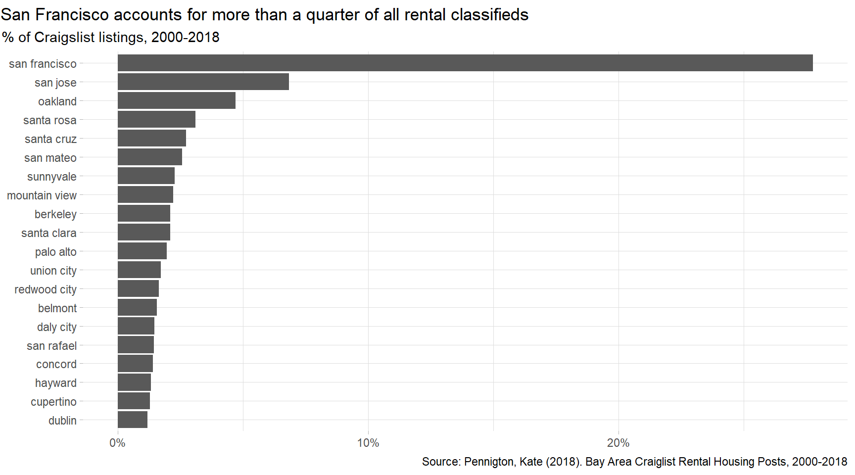
Make a plot that shows the evolution of median prices in San Francisco for 0, 1, 2, and 3 bedrooms listings.
median_per_bed <- rent %>%
  filter(beds <= 3, city == "san francisco") %>%
  group_by(beds, year) %>%
  summarize(median_price = median(price))

ggplot(median_per_bed, aes(x=year, y=median_price, color = factor(beds))) +
  geom_line() +
  facet_wrap(~beds, nrow = 1) +
  labs(
    title = "San Francisco rents have steadily been increasing",
    subtitle = "0 to 3-bed listings, 2000-2018",
    x=NULL,
    y=NULL,
    caption = "Source: Pennigton, Kate (2018). Bay Area Craiglist Rental Housing Posts, 2000-2018"
  ) +
  xlim(2003,2018) +
  theme_light() +
  theme(legend.position="none") +
  theme(plot.title = element_text(hjust = 0))+
  theme(plot.subtitle = element_text(hjust = 0)) +
  theme(strip.text.x = element_text(colour = "black")) +
  theme(panel.border = element_rect(color = "black", fill = NA, size = 0.5)) +
  theme(strip.background = element_rect(color = "black", size = 0.5))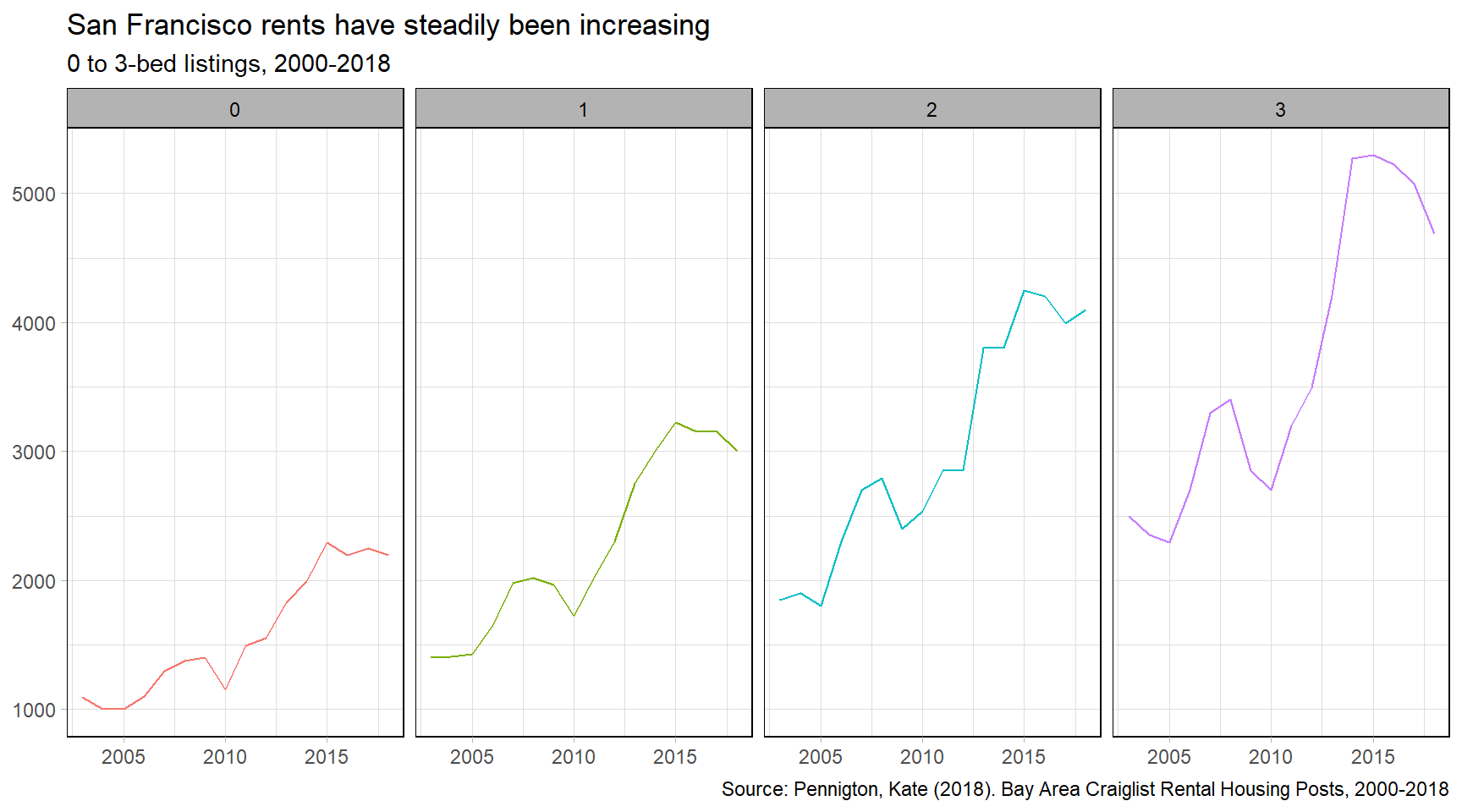
Finally, make a plot that shows median rental prices for the top 12 cities in the Bay area.
cities_to_include <- rent %>%
  group_by(city) %>%
  summarize(number_ads = n()) %>%
  slice_max(order_by = number_ads, n=12)

cities_to_include <- cities_to_include$city

median_per_bed <- rent %>%
  filter(beds == 1, city %in% cities_to_include) %>%
  group_by(city, year) %>%
  summarize(median_price = median(price))

ggplot(median_per_bed, aes(x=year, y=median_price, color = factor(city))) +
  geom_line() +
  facet_wrap(~city, nrow = 3) +
  labs(
    title = "Rental prices for 1-bedroom flats in the Bay Area",
    x=NULL,
    y=NULL,
    caption="Source: Pennigton, Kate (2018). Bay Area Craiglist Rental Housing Posts, 2000-2018"
  ) +
  theme_light() +
  theme(legend.position="none") +
  theme(plot.title = element_text(hjust = 0)) +
  theme(strip.text.x = element_text(colour = "black")) +
  theme(panel.border = element_rect(color = "black", fill = NA, size = 0.5)) +
  theme(strip.background = element_rect(color = "black", size = 0.5))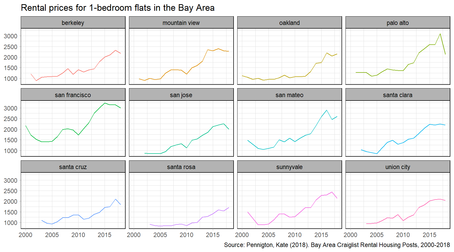
What can you infer from these plots? Don’t just explain what’s in the graph, but speculate or tell a short story (1-2 paragraphs max).
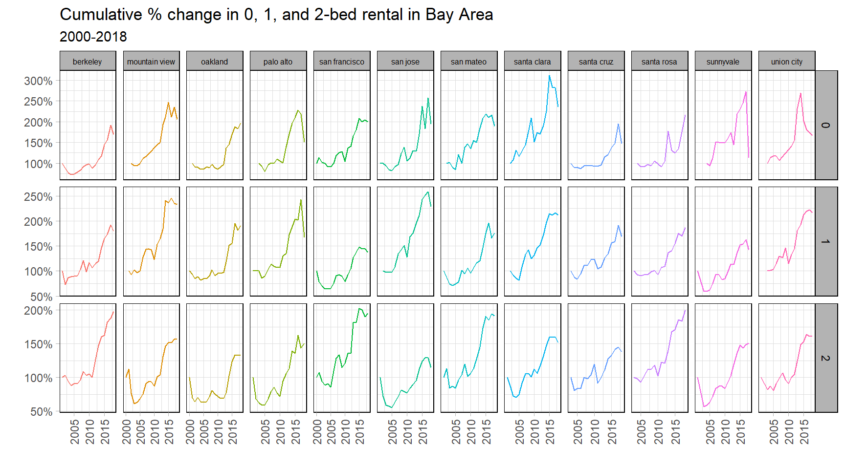
Looking at the graphs from the last exercise we can see that rental prices have increased since the year 2000. While one major cause could be inflation, it is also true that large tech companies have increased the attractiveness of the Bay Area making living there more expensive.
The figures also reveal that there has been a decline in the growth rate (or even negative growth) in the median rent after 2015. It could be due to the fact that more and more people are leaving California as the boom seems to lose momentum. A CNBC video outlines the reasons for this exodus of people.
Challenge 1: Replicating a chart
You have to create a graph that calculates the cumulative % change for 0-, 1-1, and 2-bed flats between 2000 and 2018 for the top twelve cities in Bay Area, by number of ads that appeared in Craigslist.
cities_to_include <- rent %>%
  group_by(city) %>%
  summarize(number_ads = n()) %>%
  slice_max(order_by = number_ads, n=12)

cities_to_include <- cities_to_include$city

filtered_rent <- rent %>%
  filter(beds <= 2, city %in% cities_to_include) %>%
  group_by(year, city, beds) %>%
  summarise(median_price =median(price)) %>%
  ungroup()

sorted <- filtered_rent %>%
  arrange(beds, city, year)

rent_change <- sorted %>%
  group_by(beds, city) %>%
  mutate(change_per_year = (median_price/(median_price[1L])))

ggplot(rent_change, aes(x=year, y = change_per_year, color = factor(city))) +
  geom_line() +
  facet_grid(beds~city, scales = "free") +
  labs(
    title = "Cumulative % change in 0, 1, and 2-bed rental in Bay Area",
    subtitle = "2000-2018",
    x="",
    y=""
  ) +
  ylim(0,250) +
  theme_light() +
  theme(legend.position="none")+
  theme(axis.text.x = element_text(angle = 90, vjust = 0.5, hjust=1)) +
  theme(strip.text.x = element_text(size = 6)) +
  scale_y_continuous(labels = scales::percent) +
  theme(strip.text = element_text(colour = "black")) +
  theme(panel.border = element_rect(color = "black", fill = NA, size = 0.5)) +
  theme(strip.background = element_rect(color = "black", size = 0.5))