Pre-Course Assignment

The goal is to test your software installation, to demonstrate
competency in Markdown, and in the basics of ggplot.
Task 2: gapminder country comparison
glimpse(gapminder)## Rows: 1,704
## Columns: 6
## $ country <fct> "Afghanistan", "Afghanistan", "Afghanistan", "Afghanistan", …
## $ continent <fct> Asia, Asia, Asia, Asia, Asia, Asia, Asia, Asia, Asia, Asia, …
## $ year <int> 1952, 1957, 1962, 1967, 1972, 1977, 1982, 1987, 1992, 1997, …
## $ lifeExp <dbl> 28.801, 30.332, 31.997, 34.020, 36.088, 38.438, 39.854, 40.8…
## $ pop <int> 8425333, 9240934, 10267083, 11537966, 13079460, 14880372, 12…
## $ gdpPercap <dbl> 779.4453, 820.8530, 853.1007, 836.1971, 739.9811, 786.1134, …head(gapminder, 20) # look at the first 20 rows of the dataframe## # A tibble: 20 × 6
## country continent year lifeExp pop gdpPercap
## <fct> <fct> <int> <dbl> <int> <dbl>
## 1 Afghanistan Asia 1952 28.8 8425333 779.
## 2 Afghanistan Asia 1957 30.3 9240934 821.
## 3 Afghanistan Asia 1962 32.0 10267083 853.
## 4 Afghanistan Asia 1967 34.0 11537966 836.
## 5 Afghanistan Asia 1972 36.1 13079460 740.
## 6 Afghanistan Asia 1977 38.4 14880372 786.
## 7 Afghanistan Asia 1982 39.9 12881816 978.
## 8 Afghanistan Asia 1987 40.8 13867957 852.
## 9 Afghanistan Asia 1992 41.7 16317921 649.
## 10 Afghanistan Asia 1997 41.8 22227415 635.
## 11 Afghanistan Asia 2002 42.1 25268405 727.
## 12 Afghanistan Asia 2007 43.8 31889923 975.
## 13 Albania Europe 1952 55.2 1282697 1601.
## 14 Albania Europe 1957 59.3 1476505 1942.
## 15 Albania Europe 1962 64.8 1728137 2313.
## 16 Albania Europe 1967 66.2 1984060 2760.
## 17 Albania Europe 1972 67.7 2263554 3313.
## 18 Albania Europe 1977 68.9 2509048 3533.
## 19 Albania Europe 1982 70.4 2780097 3631.
## 20 Albania Europe 1987 72 3075321 3739.country_data <- gapminder %>%
filter(country == "Italy") # just choosing Italy, as this is where I come from
continent_data <- gapminder %>%
filter(continent == "Europe")plot1 <- ggplot(data = country_data, mapping = aes(x = year, y = lifeExp))+
geom_point() +
geom_smooth(se = FALSE)+
NULL plot1 <- plot1 +
labs(title = "Life Expectancy in Italy from 1952 to 2007",
x = "Year",
y = "Life Expectancy") +
NULL
plot1## `geom_smooth()` using method = 'loess' and formula 'y ~ x'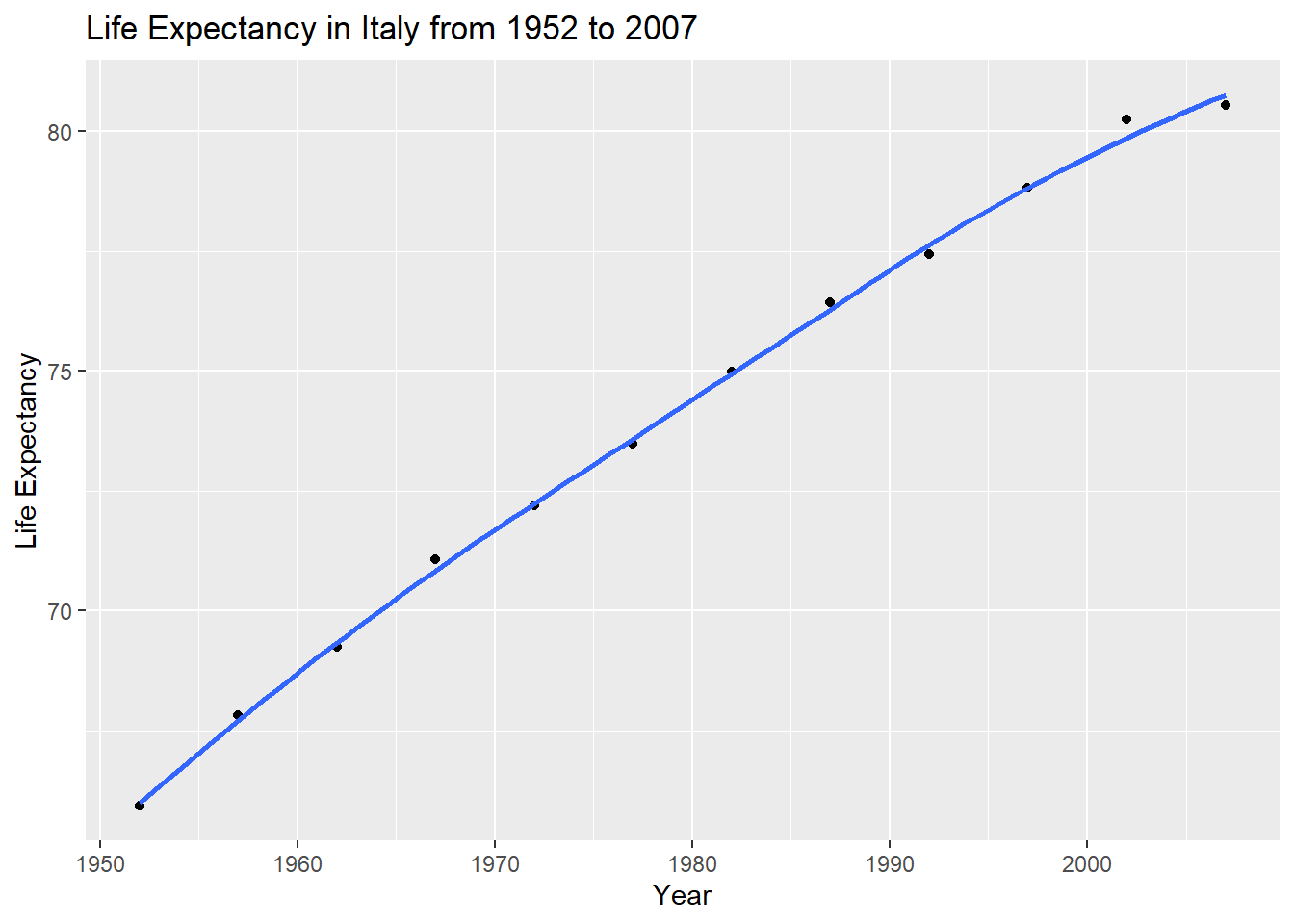
 ggplot(data = continent_data, mapping = aes(x =  year, y = lifeExp  , colour = country, group = country))+
  geom_point() +
  geom_smooth(se = FALSE) +
  NULL +
  ggtitle("Life Expectancy in Europe from 1952 to 2007")
## `geom_smooth()` using method = 'loess' and formula 'y ~ x'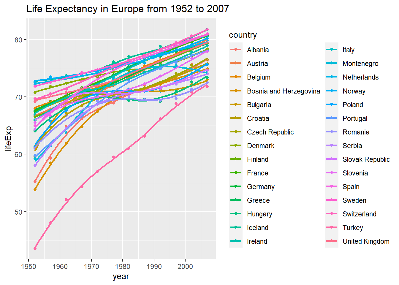
ggplot(data = gapminder , mapping = aes(x = year, y = lifeExp, colour= country))+
  geom_point() +
  geom_smooth(se = FALSE) +
  facet_wrap(~continent) +
  theme(legend.position="none") + #remove all legends
  NULL
## `geom_smooth()` using method = 'loess' and formula 'y ~ x'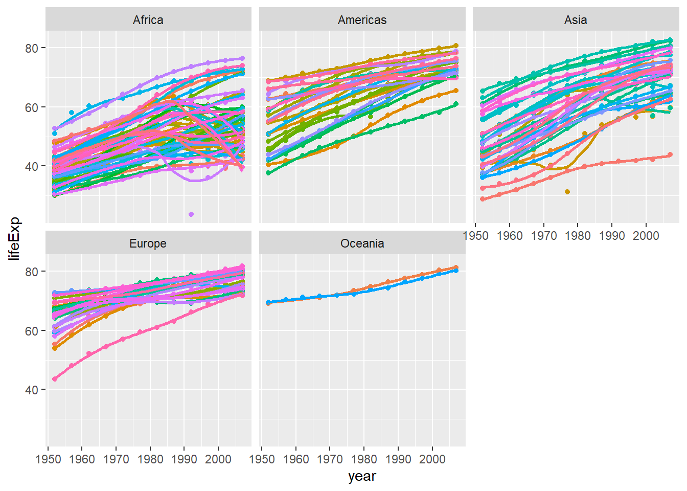
With only minor exemptions (e.g. bump in Europe in the 80s, probably Baltic states), it is visible that life expectancy in the Americas, Europe and Oceania has increased fairly steadily. This data supports the common believe, that advancements in medicine and hygiene, stable nutrition supply, less wars and overall enhancements in quality of life have contributed to an increase in life expectancy.
In Asia and Africa, however, there is once again an overall trend to increasing life expectancy but fluctuations and exemptions are more common. Especially in some African countries we see a sharp decline in life expectancy starting from the 80s and 90s. It can be speculated that this is due to epidemics - especially HIV – but also due to civil wars or famines. The average life expectancy in Asia and Africa reached in 2007 is well below that of Europe and Oceania. The standard deviation is also higher, which leads to the conclusion that there are major difference among single countries.
Task 3: Brexit vote analysis
# read data directly off github repo
brexit_results <- read_csv("https://raw.githubusercontent.com/kostis-christodoulou/am01/master/data/brexit_results.csv")


glimpse(brexit_results)
## Rows: 632
## Columns: 11
## $ Seat <chr> "Aldershot", "Aldridge-Brownhills", "Altrincham and Sale W…
## $ con_2015 <dbl> 50.592, 52.050, 52.994, 43.979, 60.788, 22.418, 52.454, 22…
## $ lab_2015 <dbl> 18.333, 22.369, 26.686, 34.781, 11.197, 41.022, 18.441, 49…
## $ ld_2015 <dbl> 8.824, 3.367, 8.383, 2.975, 7.192, 14.828, 5.984, 2.423, 1…
## $ ukip_2015 <dbl> 17.867, 19.624, 8.011, 15.887, 14.438, 21.409, 18.821, 21.…
## $ leave_share <dbl> 57.89777, 67.79635, 38.58780, 65.29912, 49.70111, 70.47289…
## $ born_in_uk <dbl> 83.10464, 96.12207, 90.48566, 97.30437, 93.33793, 96.96214…
## $ male <dbl> 49.89896, 48.92951, 48.90621, 49.21657, 48.00189, 49.17185…
## $ unemployed <dbl> 3.637000, 4.553607, 3.039963, 4.261173, 2.468100, 4.742731…
## $ degree <dbl> 13.870661, 9.974114, 28.600135, 9.336294, 18.775591, 6.085…
## $ age_18to24 <dbl> 9.406093, 7.325850, 6.437453, 7.747801, 5.734730, 8.209863…# histogram
ggplot(brexit_results, aes(x = leave_share)) +
geom_histogram(binwidth = 2.5) +
labs(title = "Histogram of leave % during Brexit Vote",
subtitle = "All constituencies",
x = "leave %-share",
y = "# constituencies")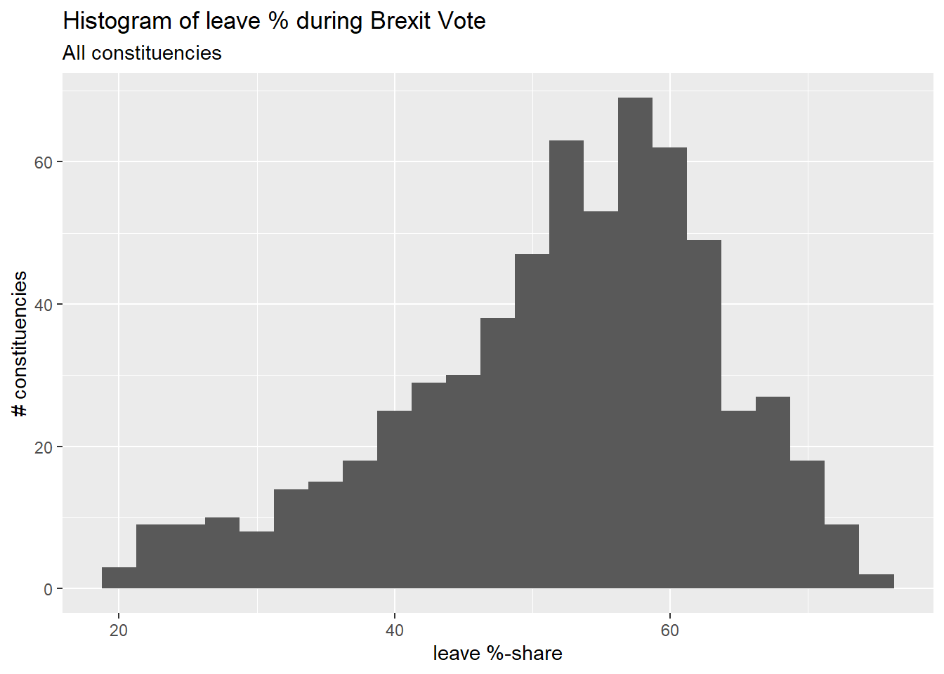
# density plot-- think smoothed histogram
ggplot(brexit_results, aes(x = leave_share)) +
  geom_density() +
  labs(title = "Density plot of leave % during Brexit Vote",
       subtitle = "All constituencies",
       x = "leave %-share",
       y = "Constituencies density")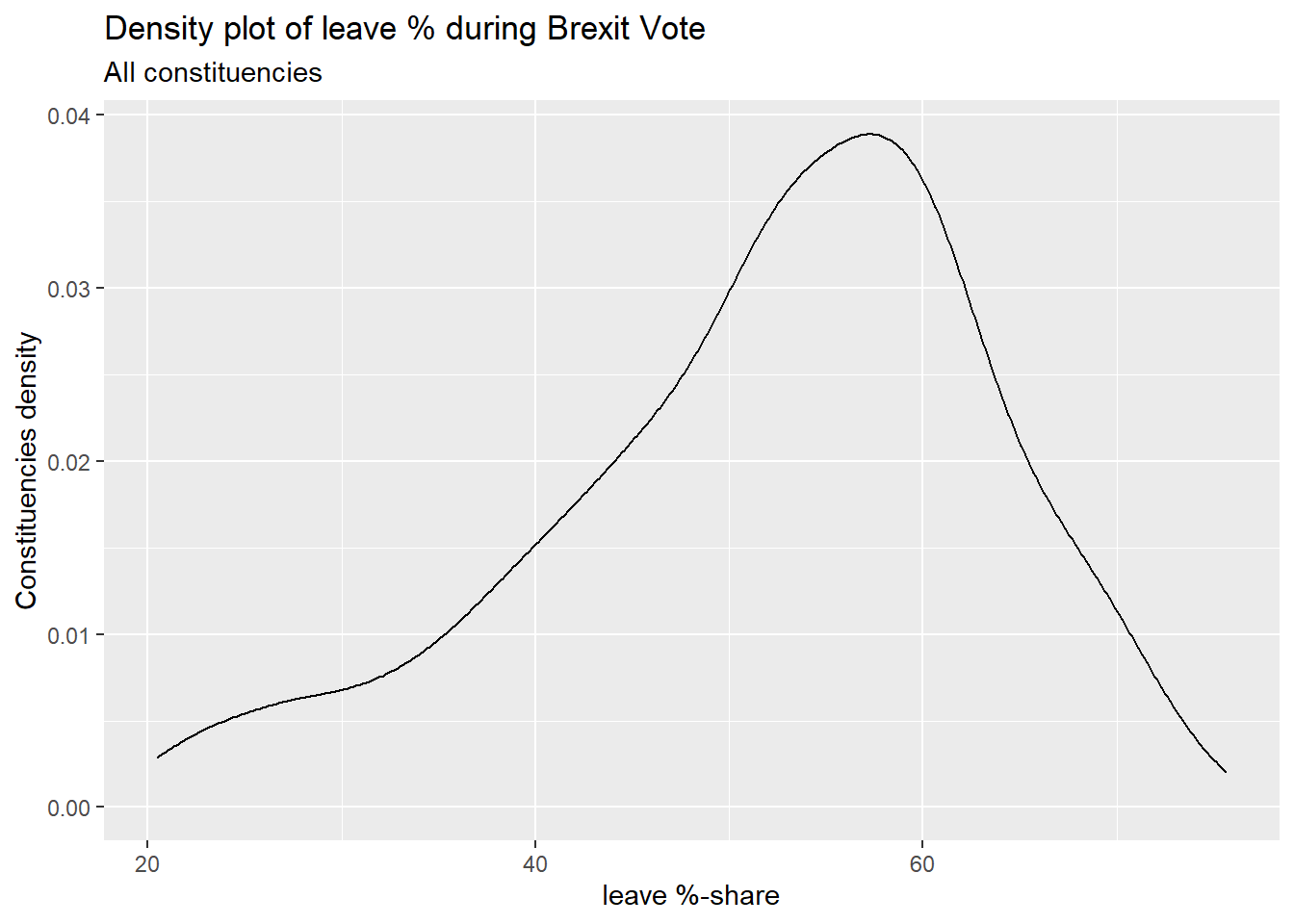
# The empirical cumulative distribution function (ECDF)
ggplot(brexit_results, aes(x = leave_share)) +
  stat_ecdf(geom = "step", pad = FALSE) +
  scale_y_continuous(labels = scales::percent) +
  labs(title = "Cumulative Distribution of leave % during Brexit Vote",
       subtitle = "All constituencies",
       x = "leave %-share",
       y = "Cumulated share of constituencies")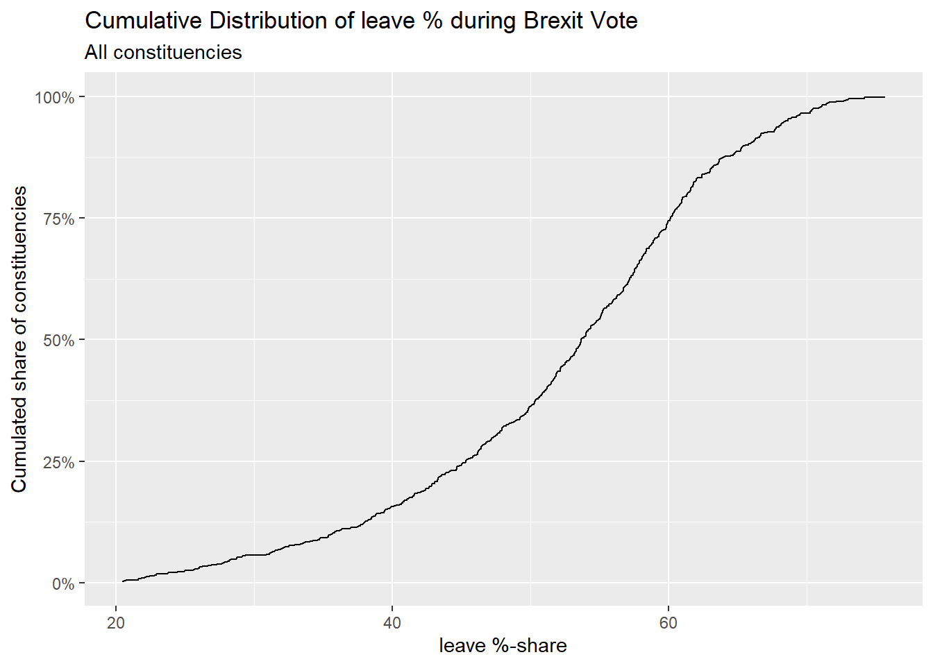
brexit_results %>%
  select(leave_share, born_in_uk) %>%
  cor()
## leave_share born_in_uk
## leave_share 1.0000000 0.4934295
## born_in_uk 0.4934295 1.0000000The correlation is almost 0.5, which shows that the two variables are positively correlated.
ggplot(brexit_results, aes(x = born_in_uk, y = leave_share)) +
  geom_point(alpha=0.3) +

  # add a smoothing line, and use method="lm" to get the best straight-line
  geom_smooth(method = "lm") +

  # use a white background and frame the plot with a black box
  theme_bw() +

  # Add titles
  labs(title = "Relationship between native borne residents and leave share",
       subtitle = "All constituencies",
       x = "native borne uk residents %-share",
       y = "leave %-share") +
  NULL
## `geom_smooth()` using formula 'y ~ x'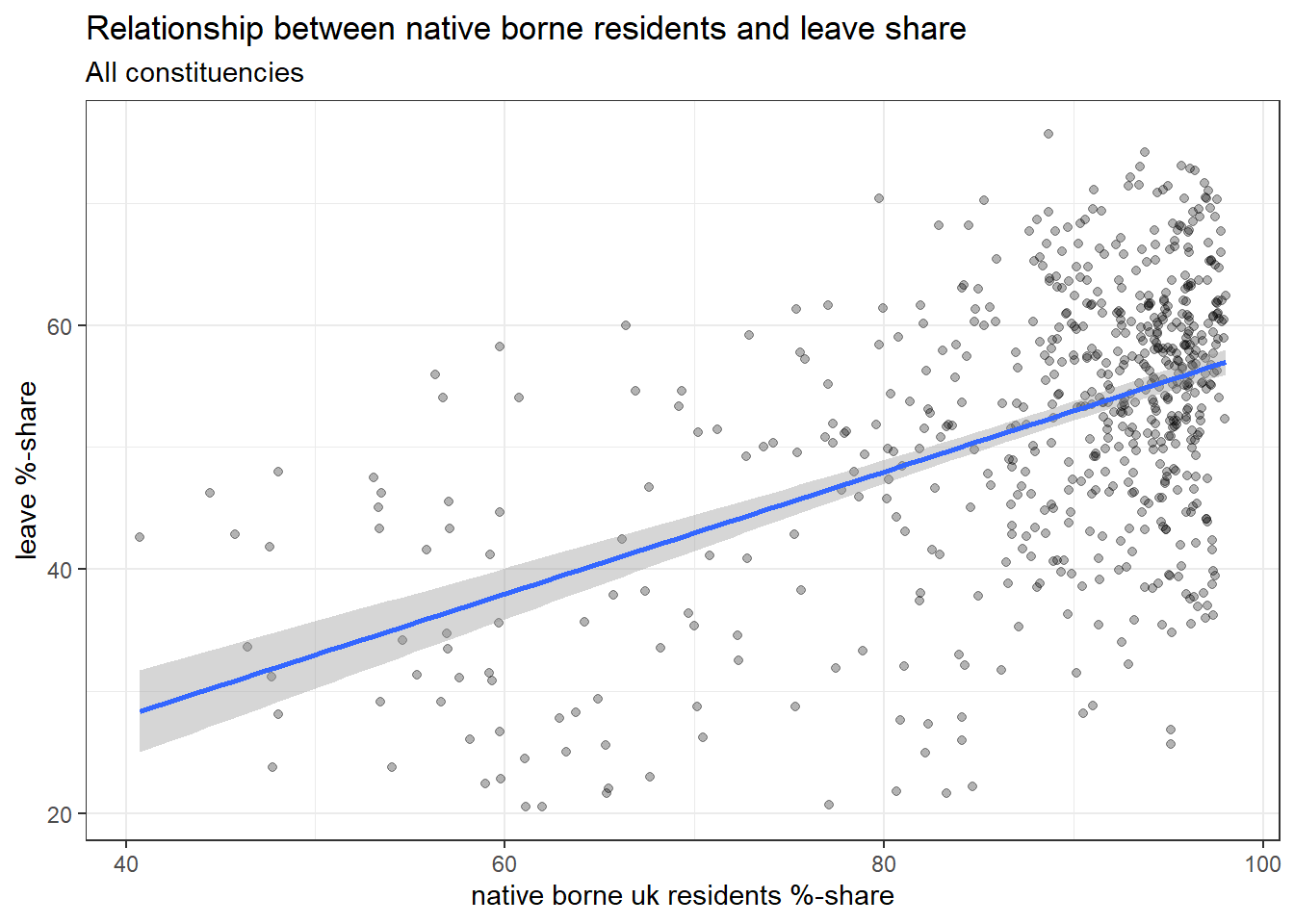
The graph shows a correlation (0.5) between the % of native born residents within a constituency and its leave %-share. A large bulk of constituencies has a born_in_uk rate of 90% and above whereby the average of leave %-share among this majority-group seems to lie around 55%. In constituencies where the % of native born residents is below 80% on the other hand, the average submitted votes would have kept the UK within the EU. These findings support the statement that patriotic, UK born citizens are more likely to oppose the EU and its regulations (among which looser immigration policies).
However, a significant standard deviation can be observed across all %-shares of native borne uk residents. In other words, this means that two constituencies with a similiar 80% “native share” have voted in favor of Brexit with 70% as well as 20%. Thus, it is suggested not to regard native born % and fear of immigration as only explanation for the Brexit outcome.
Task 4: Animal rescue incidents attended by the London Fire Brigade
url <- "https://data.london.gov.uk/download/animal-rescue-incidents-attended-by-lfb/f43b485e-fb35-419c-aa7a-fa75676e5835/Animal%20Rescue%20incidents%20attended%20by%20LFB%20from%20Jan%202009.csv"


animal_rescue <- read_csv(url,
                          locale = locale(encoding = "CP1252")) %>%
  janitor::clean_names()


glimpse(animal_rescue)
## Rows: 8,751
## Columns: 31
## $ incident_number <chr> "139091", "275091", "2075091", "2872091"…
## $ date_time_of_call <chr> "01/01/2009 03:01", "01/01/2009 08:51", …
## $ cal_year <dbl> 2009, 2009, 2009, 2009, 2009, 2009, 2009…
## $ fin_year <chr> "2008/09", "2008/09", "2008/09", "2008/0…
## $ type_of_incident <chr> "Special Service", "Special Service", "S…
## $ pump_count <chr> "1", "1", "1", "1", "1", "1", "1", "1", …
## $ pump_hours_total <chr> "2", "1", "1", "1", "1", "1", "1", "1", …
## $ hourly_notional_cost <dbl> 255, 255, 255, 255, 255, 255, 255, 255, …
## $ incident_notional_cost <chr> "510", "255", "255", "255", "255", "255"…
## $ final_description <chr> "Redacted", "Redacted", "Redacted", "Red…
## $ animal_group_parent <chr> "Dog", "Fox", "Dog", "Horse", "Rabbit", …
## $ originof_call <chr> "Person (land line)", "Person (land line…
## $ property_type <chr> "House - single occupancy", "Railings", …
## $ property_category <chr> "Dwelling", "Outdoor Structure", "Outdoo…
## $ special_service_type_category <chr> "Other animal assistance", "Other animal…
## $ special_service_type <chr> "Animal assistance involving livestock -…
## $ ward_code <chr> "E05011467", "E05000169", "E05000558", "…
## $ ward <chr> "Crystal Palace & Upper Norwood", "Woods…
## $ borough_code <chr> "E09000008", "E09000008", "E09000029", "…
## $ borough <chr> "Croydon", "Croydon", "Sutton", "Hilling…
## $ stn_ground_name <chr> "Norbury", "Woodside", "Wallington", "Ru…
## $ uprn <chr> "NULL", "NULL", "NULL", "1.00E+11", "NUL…
## $ street <chr> "Waddington Way", "Grasmere Road", "Mill…
## $ usrn <chr> "20500146", "NULL", "NULL", "21401484", …
## $ postcode_district <chr> "SE19", "SE25", "SM5", "UB9", "RM3", "RM…
## $ easting_m <chr> "NULL", "534785", "528041", "504689", "N…
## $ northing_m <chr> "NULL", "167546", "164923", "190685", "N…
## $ easting_rounded <dbl> 532350, 534750, 528050, 504650, 554650, …
## $ northing_rounded <dbl> 170050, 167550, 164950, 190650, 192350, …
## $ latitude <chr> "NULL", "51.39095371", "51.36894086", "5…
## $ longitude <chr> "NULL", "-0.064166887", "-0.161985191", …animal_rescue %>%
dplyr::group_by(cal_year) %>%
summarise(count=n())## # A tibble: 14 × 2
## cal_year count
## <dbl> <int>
## 1 2009 568
## 2 2010 611
## 3 2011 620
## 4 2012 603
## 5 2013 585
## 6 2014 583
## 7 2015 540
## 8 2016 604
## 9 2017 539
## 10 2018 610
## 11 2019 604
## 12 2020 758
## 13 2021 885
## 14 2022 641animal_rescue %>%
count(cal_year, name="count")## # A tibble: 14 × 2
## cal_year count
## <dbl> <int>
## 1 2009 568
## 2 2010 611
## 3 2011 620
## 4 2012 603
## 5 2013 585
## 6 2014 583
## 7 2015 540
## 8 2016 604
## 9 2017 539
## 10 2018 610
## 11 2019 604
## 12 2020 758
## 13 2021 885
## 14 2022 641animal_rescue %>%
group_by(animal_group_parent) %>%
#group_by and summarise will produce a new column with the count in each animal group
summarise(count = n()) %>%
# mutate adds a new column; here we calculate the percentage
mutate(percent = round(100*count/sum(count),2)) %>%
# arrange() sorts the data by percent. Since the default sorting is min to max and we would like to see it sorted
# in descending order (max to min), we use arrange(desc())
arrange(desc(percent))## # A tibble: 28 × 3
## animal_group_parent count percent
## <chr> <int> <dbl>
## 1 Cat 4232 48.4
## 2 Bird 1803 20.6
## 3 Dog 1341 15.3
## 4 Fox 455 5.2
## 5 Unknown - Domestic Animal Or Pet 215 2.46
## 6 Horse 201 2.3
## 7 Deer 152 1.74
## 8 Unknown - Wild Animal 102 1.17
## 9 Squirrel 75 0.86
## 10 Unknown - Heavy Livestock Animal 50 0.57
## # … with 18 more rowsanimal_rescue %>%
#count does the same thing as group_by and summarise
# name = "count" will call the column with the counts "count" ( exciting, I know)
# and 'sort=TRUE' will sort them from max to min
count(animal_group_parent, name="count", sort=TRUE) %>%
mutate(percent = round(100*count/sum(count),2))## # A tibble: 28 × 3
## animal_group_parent count percent
## <chr> <int> <dbl>
## 1 Cat 4232 48.4
## 2 Bird 1803 20.6
## 3 Dog 1341 15.3
## 4 Fox 455 5.2
## 5 Unknown - Domestic Animal Or Pet 215 2.46
## 6 Horse 201 2.3
## 7 Deer 152 1.74
## 8 Unknown - Wild Animal 102 1.17
## 9 Squirrel 75 0.86
## 10 Unknown - Heavy Livestock Animal 50 0.57
## # … with 18 more rows# what type is variable incident_notional_cost from dataframe `animal_rescue`
typeof(animal_rescue$incident_notional_cost)## [1] "character"# readr::parse_number() will convert any numerical values stored as characters into numbers
animal_rescue <- animal_rescue %>%
# we use mutate() to use the parse_number() function and overwrite the same variable
mutate(incident_notional_cost = parse_number(incident_notional_cost))
# incident_notional_cost from dataframe `animal_rescue` is now 'double' or numeric
typeof(animal_rescue$incident_notional_cost)## [1] "double"animal_rescue %>%
# group by animal_group_parent
group_by(animal_group_parent) %>%
# filter resulting data, so each group has at least 6 observations
filter(n()>6) %>%
# summarise() will collapse all values into 3 values: the mean, median, and count
# we use na.rm=TRUE to make sure we remove any NAs, or cases where we do not have the incident cos
summarise(mean_incident_cost = mean (incident_notional_cost, na.rm=TRUE),
median_incident_cost = median (incident_notional_cost, na.rm=TRUE),
sd_incident_cost = sd (incident_notional_cost, na.rm=TRUE),
min_incident_cost = min (incident_notional_cost, na.rm=TRUE),
max_incident_cost = max (incident_notional_cost, na.rm=TRUE),
count = n()) %>%
# sort the resulting data in descending order. You choose whether to sort by count or mean cost.
arrange(desc(mean_incident_cost))## # A tibble: 17 × 7
## animal_group_parent mean_…¹ media…² sd_in…³ min_i…⁴ max_i…⁵ count
## <chr> <dbl> <dbl> <dbl> <dbl> <dbl> <int>
## 1 Horse 735. 596 536. 255 3480 201
## 2 Cow 599. 436 451. 260 1560 9
## 3 Unknown - Wild Animal 422. 333 318. 260 2296 102
## 4 Deer 421. 339 276. 260 2340 152
## 5 Fox 382. 339 200. 255 2034 455
## 6 Snake 375. 352 122. 260 704 20
## 7 Unknown - Heavy Livestock Anim… 374. 260 263. 255 1560 50
## 8 Sheep 355. 339 114. 255 596 7
## 9 Dog 353. 326 182. 0 3168 1341
## 10 Cat 351. 326 163. 0 3912 4232
## 11 Bird 349. 328 138. 255 1788 1803
## 12 Unknown - Domestic Animal Or P… 331. 298 119. 255 1300 215
## 13 cat 329. 310. 87.4 260 596 20
## 14 Squirrel 318. 328 55.6 255 678 75
## 15 Hamster 317. 290 92.5 260 652 17
## 16 Rabbit 315. 330. 34.4 255 364 16
## 17 Ferret 314. 336 41.1 260 364 10
## # … with abbreviated variable names ¹mean_incident_cost, ²median_incident_cost,
## # ³sd_incident_cost, ⁴min_incident_cost, ⁵max_incident_costMedian usually lower, this lets us conclude that we have outliers on the top end of the cost range (single animals very difficult to rescue).
# base_plot
base_plot <- animal_rescue %>%
  group_by(animal_group_parent) %>%
  filter(n()>6) %>%
  ggplot(aes(x=incident_notional_cost))+
  facet_wrap(~animal_group_parent, scales = "free")+
  theme_bw()

base_plot + geom_histogram()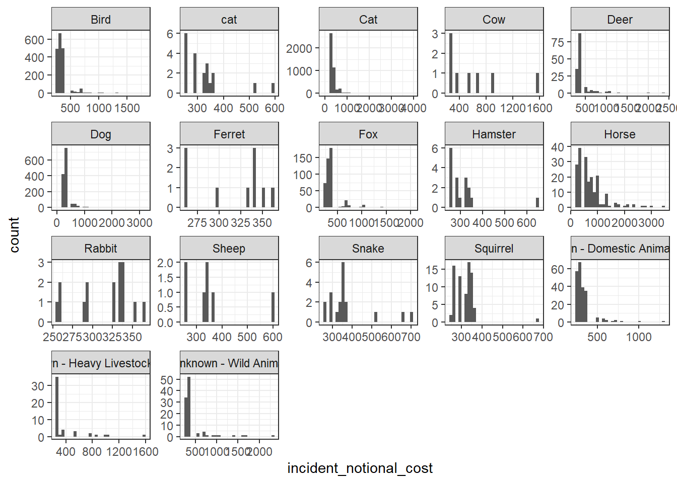
base_plot + geom_density()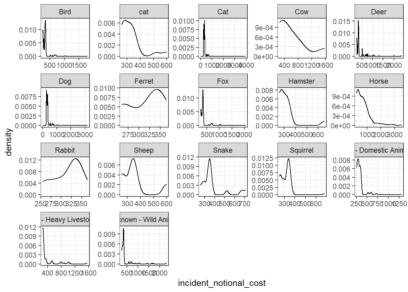
base_plot + geom_boxplot()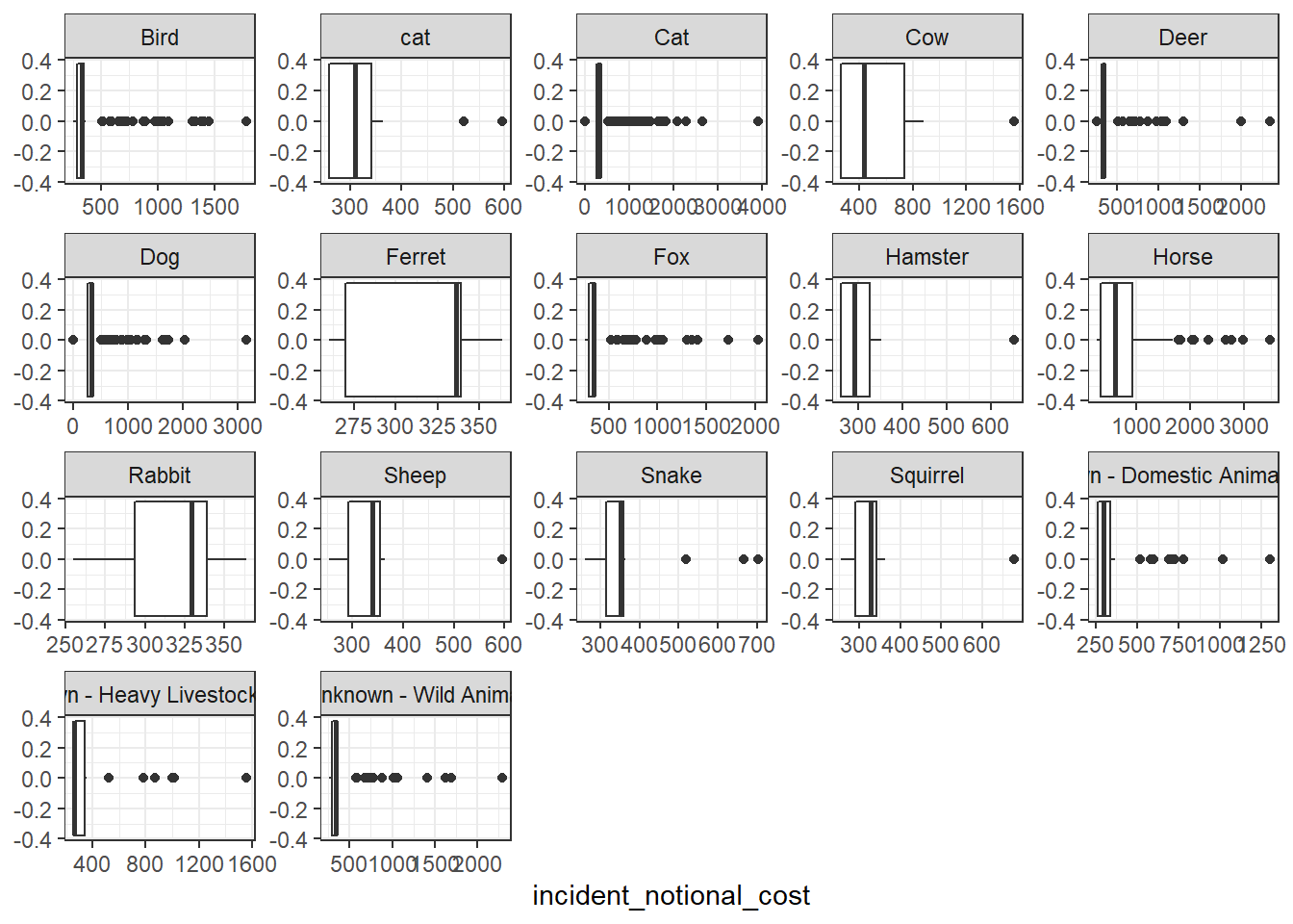
base_plot + stat_ecdf(geom = "step", pad = FALSE) +
  scale_y_continuous(labels = scales::percent)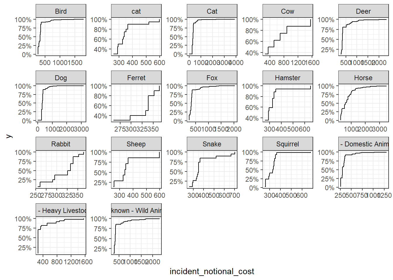
Variability is best shown in the boxplot graph as single outliers get lost in the other graphs due to the significant number of observations. As expected, large animals such as horses, cows, and deer are on average the most expensive to rescue. It is speculated that it takes more working-hours and machinery to recover heavier animals. While the minimal cost is similiar across the categories, the maximum cost seams to have some positive correlation with animal size. Correspondingly, the sd is significant in these categories, with the maximum value as high as 10x the median rescue cost. Animals such as Rabbits and Ferrets have the least outliers, a fact that could lead to the conclusion that the rescue effort for these animals is fairly predictable.